Understanding LDBC SNB: Benchmark’s Query Generation and Execution

Following our previous discussion on LDBC data generation, this blog post primarily focuses on how the query within the SNB Workload is created, and how the Driver executes the workload during performance testing.

Workload

After the preparation phase of the benchmark test, three types of data are generated:

• Dataset: used for Data from initial import
• Update Streams: used for real-time updates by the Driver during the performance testing phase
• Parameters: used for the Driver's read requests during the performance testing phase

Write Query

Given the complexity of the data generated by SNB, it is not feasible to generate update requests in real-time during performance testing through the SNB Driver. Therefore, the data for real-time updates is actually generated by DataGen. As we mentioned in the previous post, when using LDBC, DataGen needs to specify how long the data is to be generated for, and from which year social activities begin. DataGen will split all the data based on timestamps, using 90% of the data as the Dataset, and the remaining 10% as Update Streams for subsequent write requests.

For all write requests, DataGen will schedule the time of execution for the update query, and generate the related update parameters into a JSON file. We will explain later why it is necessary to specify the query scheduling time.

Read Query

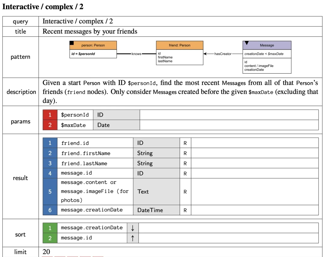
The read requests in SNB are divided into two main categories: 14 complex read-only queries and 7 short read-only queries. Complex read queries start with a given person, querying the relevant information within a one-hop or two-hop subgraph. For example, the query pattern of Interactive Complex 9 (IC9) is as follows: given a starting person to retrieve the 20 most recent messages created by this person's friends or friends of friends, as shown below.

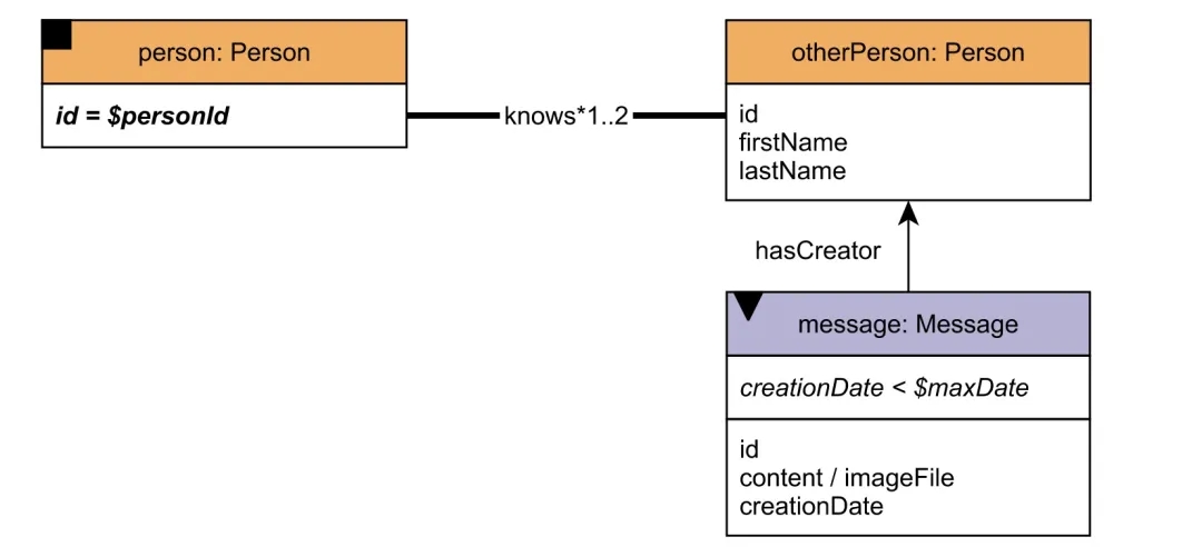
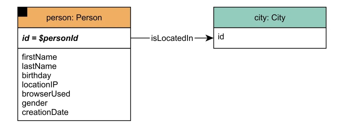
Short read queries are divided into two categories: one is to query a person’s name, age, and other information, or the friends of this person and the messages sent by these friends. The other is to retrieve the message’s sender and the related information, similar to the diagram below.

The complete request description can be found in Chapters 6.1 and 6.2 of "The LDBC Social Network Benchmark Specification".

Request Parameters

In addition to Dataset and Update Streams, DataGen also generates parameters for different read requests, such as the starting PersonId for IC9 above. To ensure the results of performance testing to be reliable, SNB requests that the parameters generated for read requests meet the following properties:

1. Query time has an upper limit: The data involved in Complex Read and Short Read requests will vary depending on the starting point, but from a macro perspective, the subgraphs they query are finite, so there will be a reasonable range for their query time.
2. Query execution time meets a stable distribution: The query data volume will vary for different starting points of the same read request, but the final query time distribution is stable.
3. Identical logical plan: Given a query, no matter how different the starting points are, the logical query plan generated by the optimizer is the same. This property ensures that each query can test some technical difficulties in the graph database, such as a large number of JOINs, cardinality estimation, etc..

The first two properties are relatively easy to understand, but what about the last one? We all know that an excellent optimizer will determine the JOIN order during actual execution based on query parameters. Even for the same query pattern, the final execution plan can vary greatly due to different query parameters. Let's see how DataGen selects parameters to enable the same query to ultimately adopt the same query plan.

Firstly, it is known that the query data volume and query time are strongly correlated. For each query pattern, LDBC has an ideal execution plan during its design, in which the data volume can be pre-calculated based on the starting point.

Take Complex 2 as an example.

When retrieving the most recent 20 messages sent by a given person's friends, the ideal query plan is as follows.

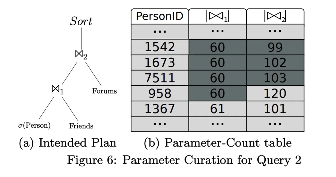
For this ideal execution plan, we can preprocess to get the number of rows of the JOIN intermediate result for each starting point. For example, for the starting point of PersonID=1542, the number of intermediate results of the two JOINs are 60 and 99 respectively. Ultimately, for each Query, a table of the starting point and the number of rows of the intermediate JOIN result, called the Parameter-Count table, will be generated.

The Parameter-Count table is generated by DataGen during the data generation process. With this table, selecting parameters actually turns into choosing the most similar rows in the table. The method used in this step is a greedy heuristic search: first, select the most similar rows based on the number of Join1 intermediate results (rows where Join1 value is 60), then select from these rows based on the number of Join2 intermediate results (resulting in rows where Join2 values are 99, 102, 103), finally filtering out PersonID 1542, 1673, 7511.

One concern that may raise is that, logically, the number of parameters to be selected, k, should be determined first, then the Parameter-Count table should be screened. Otherwise, as the paper suggests, this could lead to the final number of selected rows being less than k. This has not been investigated in depth here, but the overall approach is reasonable.

Through the above steps, for each Query type, several most similar parameters will be selected to make the query plan as similar as possible. However, a question remains, how to determine how many parameters each query needs, i.e., the quantity of different queries?

Query Mix

First of all, the LDBC SNB Interactive Workload expects the execution time ratio of Update Query, Complex Query, and Short Query during the performance test to be 10%, 50%, and 40% respectively. This ratio is designed to simulate the real load of social networks, where read requests generally far outnumber write requests, and to realistically reflect the performance of the database.

Although in the previous step, DataGen ensures that the execution times of different parameters in the same query were similar. However, there are huge differences in the data volume and execution data of different queries. Therefore, in order to avoid a certain type of query playing a decisive role in the final test results, the quantity of different types of queries needs to be carefully designed.

The SNB Interactive Workload mainly believes that the Complex Read Query should dominate the performance test scores. The number of Complex Read Queries is determined by the number of Update Queries, as shown in the table below.

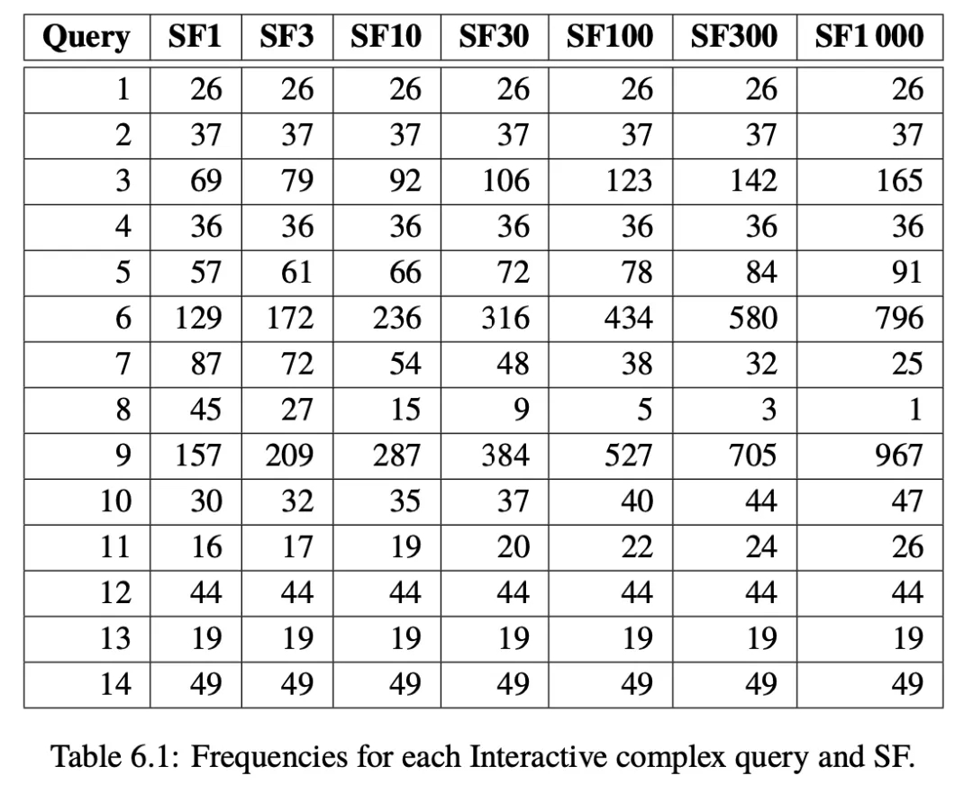
For example, in SF100, a Complex Read Query 9 should be executed after every 527 Update Queries. As mentioned before, the scheduling time for each Update Query has been determined by DataGen, so the scheduling time for each Complex Read is also set. Note that the scheduling time can be understood as a relative time compared to the start time of the performance test, which will actually be affected by the SNB Driver parameters. The reason it is a scheduling time rather than an execution time is that the database being tested may already be fully loaded or unresponsive, causing a Query that has reached its scheduling time to be unable to execute in a timely manner.

This is where we can understand why SNB claims that its test results are repeatable. The key lies in the deterministic data generated by DataGen. Once the scheduling time of the Update Query is determined, it also sets the scheduling time of the Complex Read Query, thereby ensuring the repeatability of its performance test results. Understanding this is crucial for subsequent comprehension of performance test results and relevant parameters of the SNB Driver.

Meanwhile, Short Queries are interspersed after each Complex Query. As mentioned before, Short Queries fall into two major categories: querying person-related information or message-related information. To be precise, different types of Complex Queries may return different information. Based on the results of the Complex Query, a type will be selected from the Short Queries, and the result of the Complex Read, such as identifiers of Person or Message, will be used as parameters for the Short Query.

After a Short Query is scheduled, another Short Query may be scheduled subsequently, with the probability decreasing each time. That is, a string of Short Queries may be scheduled after a Complex Query, referred to as Short Read Random Walk in the paper. Different Queries may trigger different types of Short Queries, as shown in the table below. For instance, only IS1, IS2 and IS3 can be triggered after IC10.

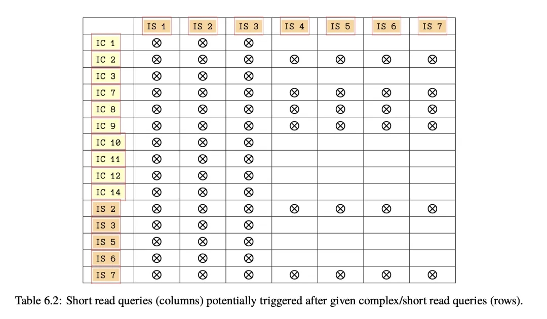
IC in the table stands for Interactive Complex query, and IS stands for Interactive Short query.

Unlike Complex Queries, the scheduling time of Short Queries is dynamically determined by the Driver based on the completion time of the Complex Read it depends on. However, the number of Short Queries triggered is determined by the aforementioned probability. Since all the random generators used during the performance testing process are the same, the proportion and order of all Queries in the entire benchmark testing process are fixed.

Driver The Driver relies on the Dataset, Update Streams, and Parameters generated by DataGen, and it mainly accomplishes two tasks:

• Validate: to check the correctness of the database
• Benchmark: to test the performance of the database

Validation is relatively straightforward. Based on the Update Streams and Parameters, several parameters are generated for validation. To verify the correctness of the database results, validation depends on executing queries in a determined order, so it can only be performed in a single thread. The Driver will ultimately output whether the database has passed the validation.

Benchmarking, on the other hand, generates a determined Workload, including an Operation sequence that contains Query and corresponding scheduling times, based on the Dataset, Update Streams, Parameters, and relevant configurations. According to the scheduling times, Workload is sent in sequence to the database being tested, while also their scheduling times, start execution times, and end execution times are saved, ultimately outputting a performance report.

The Driver is mainly composed of the Runtime, Workload, Database Connector, and Report.

Runtime & Workload

Regardless of the final performance test environment or the graph database being tested, the Workload it generates will be the same as long as the Driver's input (data and configurations) is the same. To achieve the highest throughput, the Workload is often broken down into multiple Streams. For graphs, multiple operations have dependencies, such as the existence of a friend before a friendship can be added. Therefore, the Driver supports execution of this sequence by multiple threads (controlled by the thread_count parameter), but it also needs to ensure that even with multiple threads executing, the dependencies between operations still satisfy the scheduling time relationships generated by DataGen. The principle of this part is not elaborated, but those interested can read the relevant section in the paper.

Each Operation in the Workload includes the following information:

• Query type
• Query parameters
• Scheduling time
• Expected result (used only in Validate)

As mentioned before, all the scheduling times for Update Query and Complex Query are predetermined by DataGen. The Driver sends the Query to the database for execution via the Database Connector according to the scheduling time. Obviously, if these scheduling times are all a fixed value, we cannot know the real performance of the database.

In the Driver, the parameter time_compression_ratio (default is 1) can stretch or compress the entire Workload in the time dimension. For example, a time_compression_ratio of 2.0 means that the running duration of this benchmark will become twice the default, that is, the interval time between Queries will become twice the original. Similarly, atime_compression_ratio of 0.1 means that the speed at which the Driver sends Queries is 10 times the default. In short:

• time_compression_ratio > 1, slower than default
• time_compression_ratio < 1, faster than default

Note that modifying the time_compression_ratio will not affect the ratio of different types of Queries in the Query sequence, the Query parameters, and the execution order.

Database Connector

To interface a database with SNB, vendors need to implement the corresponding Database Connector with the primary task to connect to the target database:

1. Convert the Query type and parameters of the Driver framework into the Query of the target graph database. Send the Query to the target graph database through the Database Connector.
2. This part only needs to implement several interfaces of the Driver, referring to: https://github.com/ldbc/ldbc_snb_interactive_v1_driver and the related integration documentation.

Driver Configuration

The main purpose of the benchmark is to achieve the optimal time_compression_ratio (the smaller, the higher the performance) while ensuring a timeliness rate of more than 95%. An Operation is considered timely if it is scheduled by the Driver within 1 second after the expected scheduling time:

actual_start_time − scheduled_start_time < 1 second

Moreover, a valid Benchmark takes at least two hours while the performance during the half-hour warm-up period is not included in the results.

To run a valid Benchmark, the Driver has several important parameters to adjust:

• time_compression_ratio: Adjust the execution speed of the Workload, more precisely, the expected execution speed.
• operation_count: The total number of Operations that the Driver needs to generate, modify with - time_compression_ratio, to ensure the duration of the Benchmark.
• thread_count: The size of the thread pool for executing Operations. Depending on the performance of the database to be tested, it may also be necessary to adjust the number of concurrently executing Queries.

Report

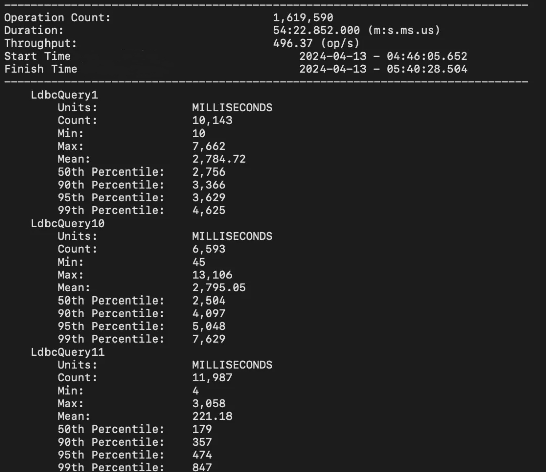
Eventually, the Driver will generate the following performance metrics:

• Start Time: When the first Operation begins.
• Finish Time: When the last Operation is completed.
• Total Run Time: The duration between Finish Time and Start Time.
• Total Operation Count: The total number of Operations, the total number of Operations executed.

The system's QPS can be obtained by Total Operation Count / Total Run Time.

For each type of Query, the Driver will also output the total number of each Query, the average, median, P95, P99 of the execution time, and the distribution of scheduling time latency.

Reference

The original intention of these articles is to help readers understand the logics of LDBC SNB as we found SNB not easily understood when we were running the testing of our own system. We may write more articles around the LDBC design topics. Please stay tuned!

• ldbc-snb-interactive-sigmod-2015.pdf (ldbcouncil.org)
• The LDBC Social Network Benchmark Specification
• GitHub - ldbc/ldbc_snb_interactive_v1_driver: Driver for the LDBC SNB Interactive workload