7 Fundamental Use Cases of Social Networks with NebulaGraph Database | EP 3

In this third episode of our series on social network analysis using graph databases, we will delve deeper into the power of this technology to uncover insights about our networks. Building upon the concepts introduced in previous episodes, such as identifying key people, determining the closeness between two users, and recommending new friends, we will now explore new techniques for pinpointing important content using common neighbors, pushing information flow based on friend relationships and geographic location, and using spatio-temporal relationship mapping to query the relationship between people. We will also look at how this technology can be used to identify the provinces visited by a group of people who intersected in time and space.

Previously on: Episode 1| Episode 2

Common Neighbor

Finding common neighbors is a very common graph database query, and its scenarios may bring different scenarios depending on different neighbor relationships and node types. The common buddy in the first two scenarios is essentially a common neighbor between two points, and directly querying such a relationship is very simple with OpenCypher.

A common neighbor between two vertices

For example, this expression can query the commonality, intersection between two users, the result may be common teams, places visited, interests, common participation in post replies, etc.:.

MATCH p = (`v0`)--()--(`v1`)
WHERE id(`v0`) == "player100" AND id(`v1`) == "player104"
RETURN p

And after limiting the type of edge, this query is limited to the common friend query.

MATCH p = (v0)--(:`follow`)--(v1)
WHERE id(v0) == "player100" AND id(v1) == "player104"
RETURN p

Common neighbors among multiple vertices: content notification

Below, we give a multi-nodes common neighbor scenario where we trigger from a post, find out all the users who have interacted on this post, and find the common neighbors in this group.

What is the use of this common neighbor? Naturally, if this common neighbor has not yet had any interaction with this article, we can recommend this article to him.

The implementation of this query is interesting.

• The first MATCH is to find the total number of people who left comments and authors on all post11 articles
• After the second MATCH, we find the number of friends of the interacting users who have participated in the article that is exactly equal to the number of users who have participated in the article, and they are actually the common friends of all the participating users.

MATCH (blog:post)<-[e]-(:player) WHERE id(blog) == "post11"
WITH blog, count(e) AS invoved_user_count
MATCH (blog:post)<-[]-(users:player)-[:`follow`]-(common_neighbor:player)
WITH toSet(collect(users)) AS users, common_neighbor, invoved_user_count
WHERE size(users) == invoved_user_count
RETURN common_neighbor

And that person is . . Tony!

+-----------------------------------------------------+
| common_neighbor                                     |
+-----------------------------------------------------+
| ("player101" :player{age: 36, name: "Tony Parker"}) |
+-----------------------------------------------------+

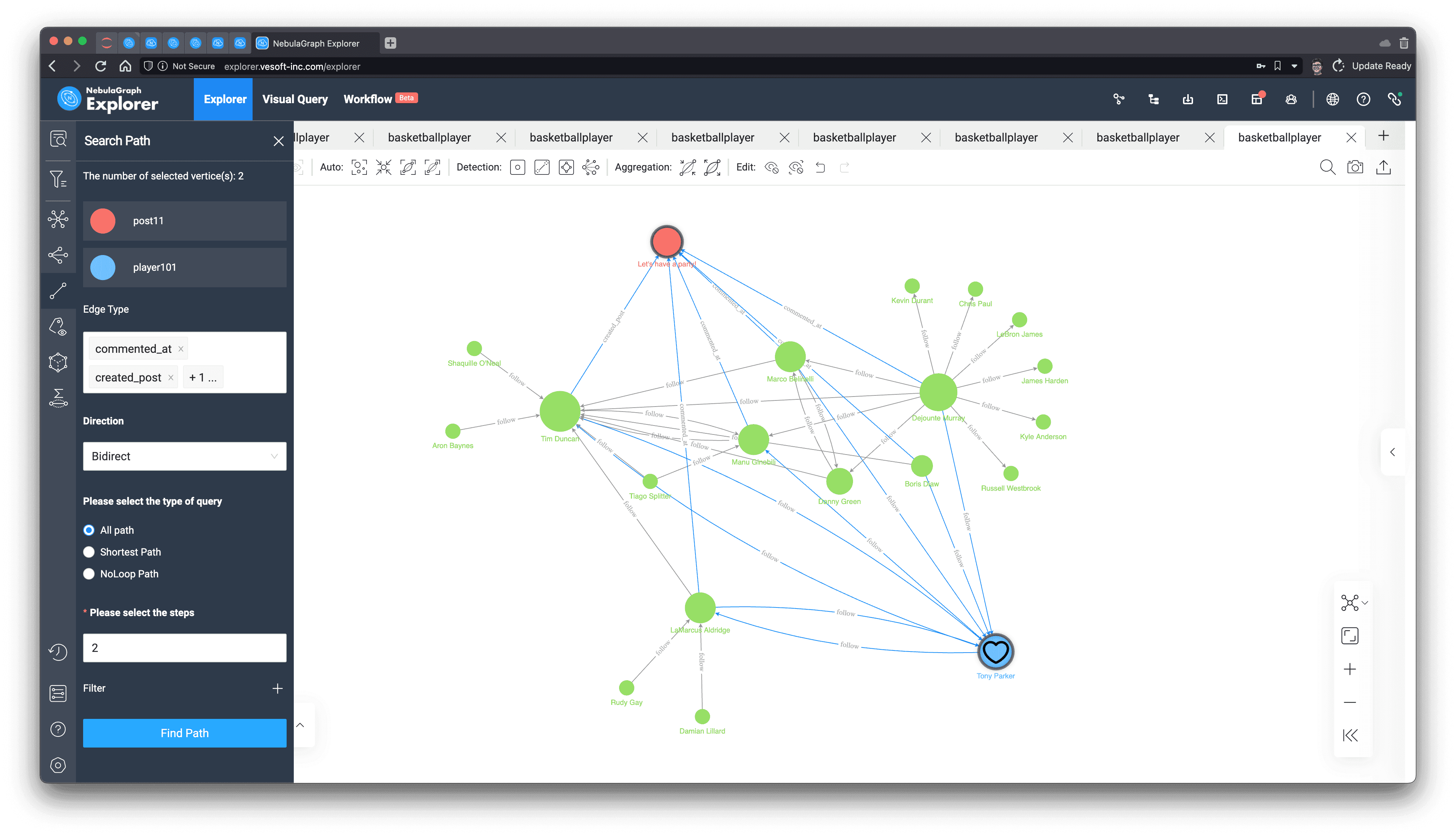
And we can easily verify it in the visualization of the query:

MATCH p=(blog:post)<-[]-(users:player)-[:`follow`]-(common_neighbor:player)
WHERE id(blog) == "post11"
RETURN p

Rendering this query, and then looking for two-way, two-hop queries between the article called "Let's have a party!" and Tony's comments, posts, and followers, we can see that all the people involved in the article are, without exception, Tony's friends, and only Tony himself has not yet left a comment on the article!

And how can a party be without Tony? Is it his surprise birthday party, Opps, shouldn't we tell him, or?

Feed Generation

I have previously written about the implementation of recommendation systems based on graph technology, in which I described that content filtering and sorting methods in modern recommendation systems can be performed on graphs. It is also highly time-sensitive. The feed generation in a SNS is quite similar but slightly different.

Content with friend engagement

The simplest and most straightforward definition of content generation may be the facebook feed of content created and engaged by people you follow.

• Content created by friends within a certain period of time
• the content of friends' comments within a certain time frame

We can use OpenCypher to express this query for the stream of information with user id player100.

MATCH (feed_owner:player)-[:`follow`]-(friend:player) WHERE id(feed_owner) == "player100"
OPTIONAL MATCH (friend:player)-[newly_commented:commented_at]->(:post)<-[:created_post]-(feed_owner:player)
    WHERE newly_commented.post_time > timestamp("2010-01-01 00:00:00")
OPTIONAL MATCH (friend:player)-[newly_created:created_post]->(po:post)
    WHERE newly_created.post_time > timestamp("2010-01-01 00:00:00")
WITH DISTINCT friend,
    collect(DISTINCT po.post.title) + collect("comment of " + dst(newly_commented))
        AS feeds WHERE size(feeds) > 0
RETURN friend.player.name, feeds

So, we can send these comments, articles to the user's feed.

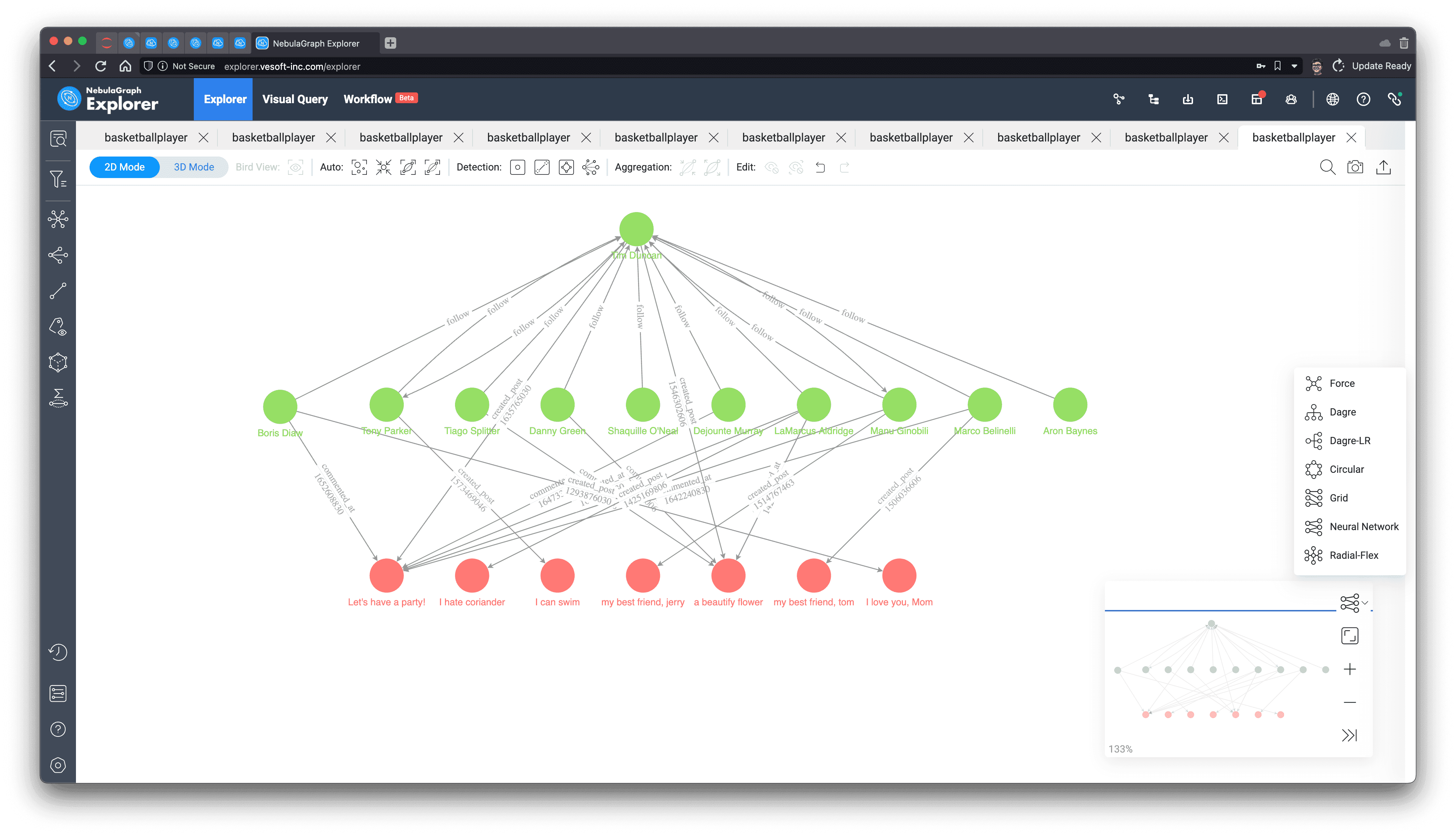
Let's also see what they look like on the graph, we output all the paths we queried:

MATCH p=(feed_owner:player)-[:`follow`]-(friend:player) WHERE id(feed_owner) == "player100"
OPTIONAL MATCH p_comment=(friend:player)-[newly_commented:commented_at]->(:post)<-[:created_post]-(feed_owner:player)
    WHERE newly_commented.post_time > timestamp("2010-01-01 00:00:00")
OPTIONAL MATCH p_post=(friend:player)-[newly_created:created_post]->(po:post)
    WHERE newly_created.post_time > timestamp("2010-01-01 00:00:00")
RETURN p, p_comment, p_post

Rendering on Explorer and selecting the "Neural Network" layout, you can clearly see the pink article nodes and the edges representing the comments.

Content of nearby friends

Let's go a step further and take geographic information(GeoSpatial) into account to get content related to friends whose addresses have a latitude and longitude less than a certain distance.

Here, we use NebulaGraph's GeoSpatial geography function, the constraint ST_Distance(home.address.geo_point, friend_addr.address.geo_point) AS distance WHERE distance < 1000000 helps us express the distance limit.

MATCH (home:address)-[:lived_in]-(feed_owner:player)-[:`follow`]-(friend:player)-[:lived_in]-(friend_addr:address)
    WHERE id(feed_owner) == "player100"
WITH feed_owner, friend, ST_Distance(home.address.geo_point, friend_addr.address.geo_point) AS distance WHERE distance < 1000000

OPTIONAL MATCH (friend:player)-[newly_commented:commented_at]->(:post)<-[:created_post]-(feed_owner:player)
    WHERE newly_commented.post_time > timestamp("2010-01-01 00:00:00")
OPTIONAL MATCH (friend:player)-[newly_created:created_post]->(po:post)
    WHERE newly_created.post_time > timestamp("2010-01-01 00:00:00")
WITH DISTINCT friend,
    collect(DISTINCT po.post.title) + collect("comment of " + dst(newly_commented))
        AS feeds WHERE size(feeds) > 0
RETURN friend.player.name, feeds

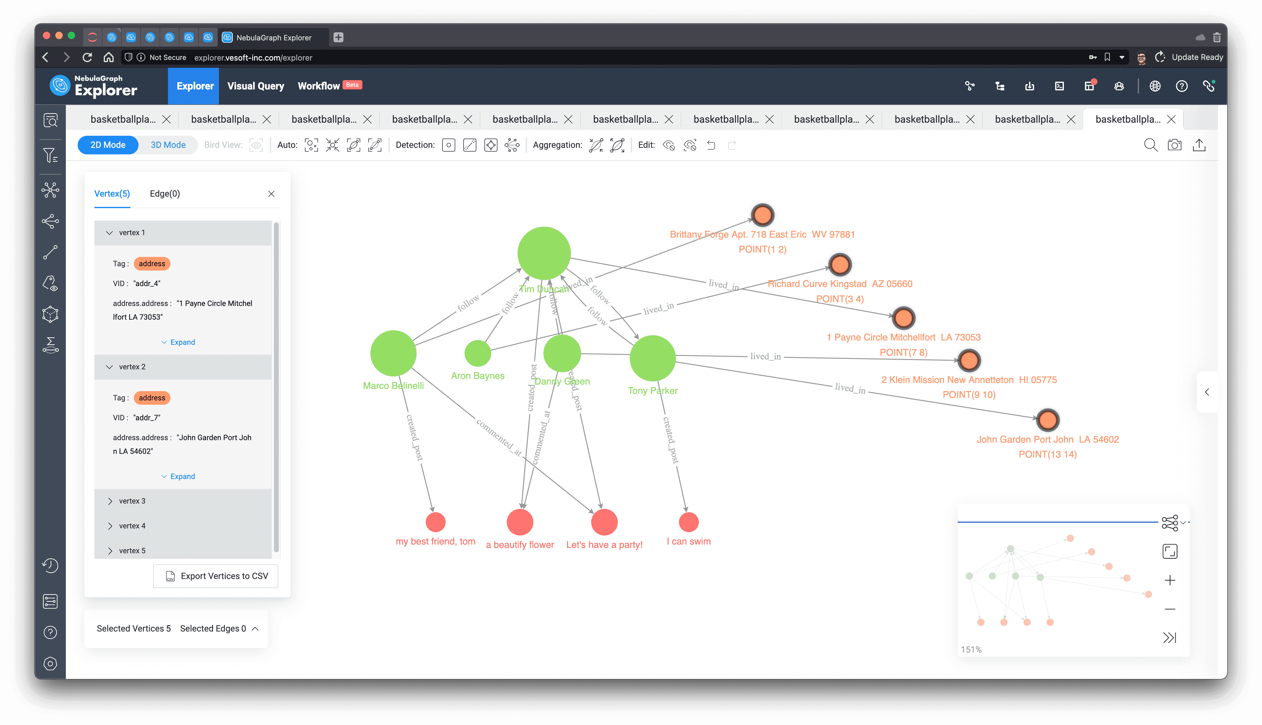
At this point, you can also see the relationship between addresses and their latitude and longitude information from the visualization of this result.

I manually arranged the nodes of the addresses on the graph according to their latitude and longitude and saw that the address (7, 8) of Tim(player100), the owner of this feed, is exactly in the middle of other friends' addresses.

Spatio-temporal relationship tracking

Spatio-temporal relationship tracking is a typical application that uses graph traversal to make the most of complicated and messy information in scenarios such as public safety, logistics, and epidemic prevention and control. When we build such a graph, we often need only simple graph queries to gain very useful insights. In this section, I'll give an example of this application scenario.

Dataset

For this purpose, I created a fake dataset by which to build a spatio-temporal relationship graph. The dataset generation program and a file that can be used directly are placed on GitHub at https://github.com/wey-gu/covid-track-graph-datagen.

It models the data as follows.

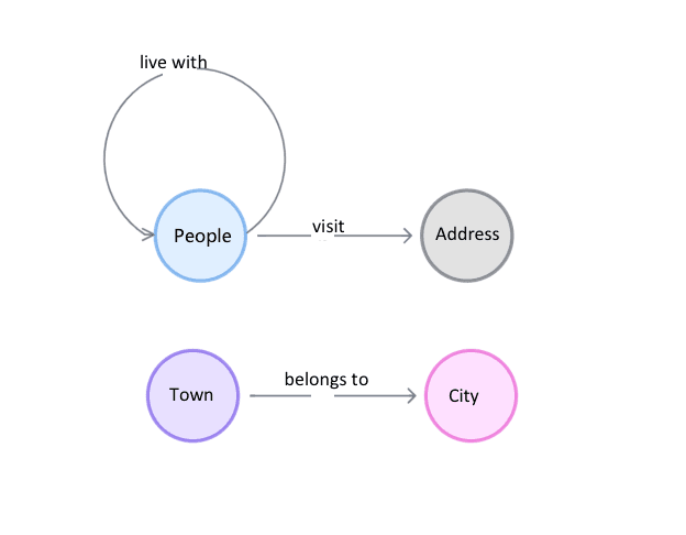
We could get the data ready in three lines in any Linux System:

# Install NebulaGraph + NebulaGraph Studio
curl -fsSL nebula-up.siwei.io/install.sh | bash -s -- v3
# Clone the dataset
git clone https://github.com/wey-gu/covid-track-graph-datagen && cd covid-track-graph-datagen
# Load the dataset into NebulaGraph
docker run --rm -ti \
    --network=nebula-net \
    -v ${PWD}/:/root \
    vesoft/nebula-importer:v3.2.0 \
    --config /root/nebula-importer-config.yaml

Then we could inspect the data from console:

~/.nebula-up/console.sh
# access console, and sse the covid_trace graph space
USE covid_trace;
# check stats
SHOW STATS

Results:

(root@nebula) [covid_trace]> SHOW STATS
+---------+------------+--------+
| Type    | Name       | Count  |
+---------+------------+--------+
| "Tag"   | "person"       | 10000  |
| "Tag"   | "address"     | 1000   |
| "Tag"   | "city"     | 341    |
| "Tag"   | "town"     | 42950  |
| "Tag"   | "state"     | 32     |
| "Tag"   | "contact" | 0      |
| "Tag"   | "district"   | 3134   |
| "Tag"   | "street"     | 667911 |
| "Edge"  | "home"     | 0      |
| "Edge"  | "visit"     | 19986  |
| "Edge"  | "live with"     | 19998  |
| "Edge"  | "belong to"     | 715336 |
| "Space" | "vertices" | 725368 |
| "Space" | "edges"    | 755320 |
+---------+------------+--------+
Got 14 rows (time spent 1087/46271 us)

Connections between two

This could be done with FIND PATH

# SHORTEST
FIND SHORTEST PATH FROM "p_100" TO "p_101" OVER * BIDIRECT YIELD PATH AS paths

# ALL PATH
FIND ALL PATH FROM "p_100" TO "p_101" OVER * BIDIRECT YIELD PATH AS paths | LIMIT 10

SHORTEST Path result:

ALL Path result:

We render all the paths visually, mark the two people at the starting node and end end, and check their shortest paths in between, and the inextricable relationship between them is clear at a glance, whether it is for business insight, public safety or epidemic prevention and control purposes, with this information, the corresponding work can progress downward like a tiger.

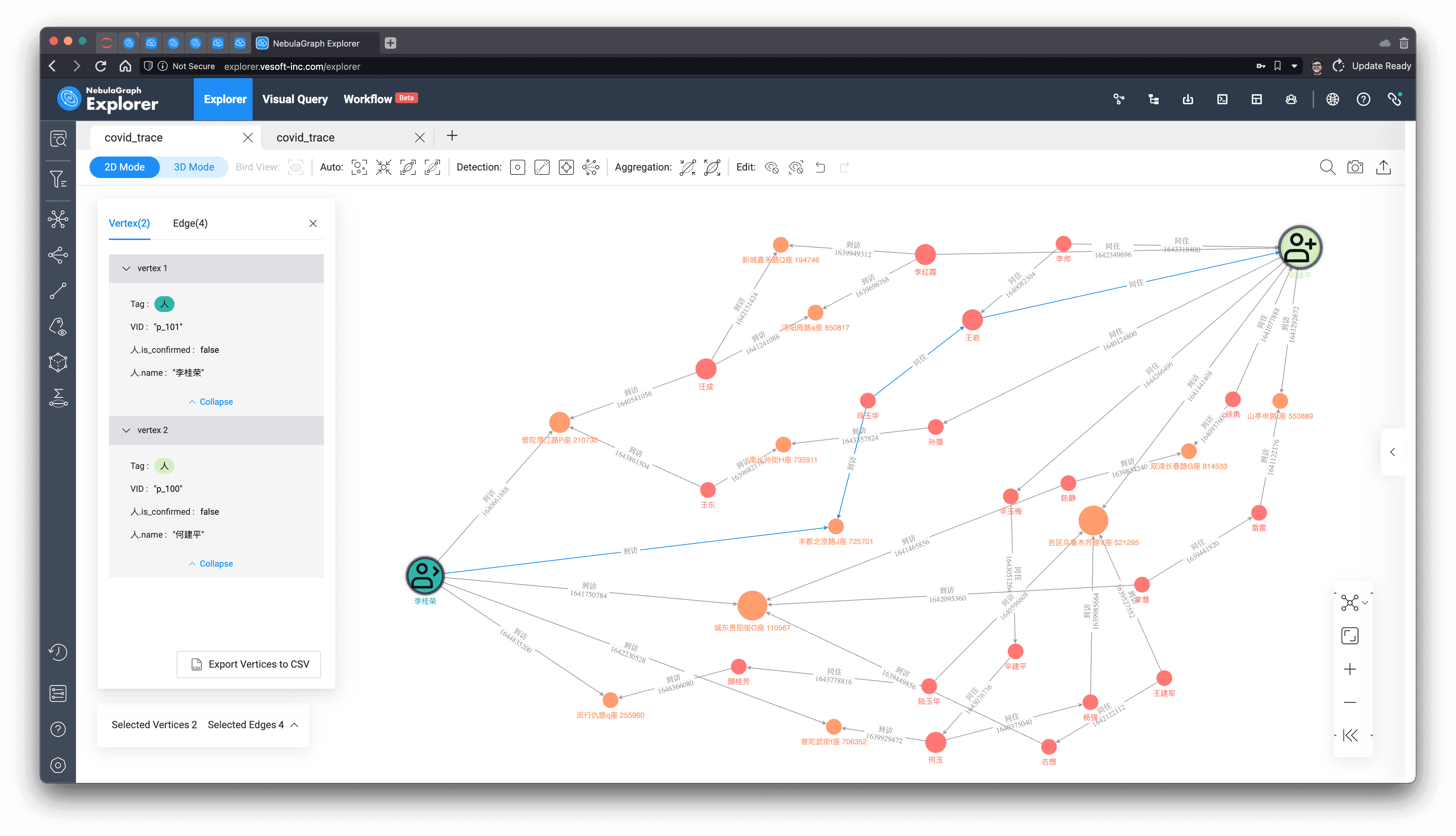
Of course, on a real world system, it may be that we only need to care about the proximity of the association between two users:

FIND SHORTEST PATH FROM "p_100" TO "p_101" OVER * BIDIRECT YIELD PATH AS paths |
    YIELD collect(length($-.paths)) AS len | YIELD coalesce($-.len[0], -1) AS len

In the result we only care about the length of the shortest path between them as: 4.

Temporal intersection of people

Further we can use graph semantics to outline any patterns with temporal and spatial information that we want to identify and query them in real time in the graph, e.g. for a given person whose id is p_101, we differ all the people who have temporal and spatial intersection with him at a given time, which means that those people also stay and visit a place within the time period in which p_101 visits those places.

MATCH (p:person)-[`visit0`:visited]->(`addr`:address)<-[`visit1`:visited]-(p1:person)
    WHERE id(p) == "p_101" AND `visit0`.`start_time` < `visit1`.`end_time`
    RETURN `addr`.address.`name`, collect(p1.person.`name`)

We obtained the following list of temporal intersection people at each visited location.

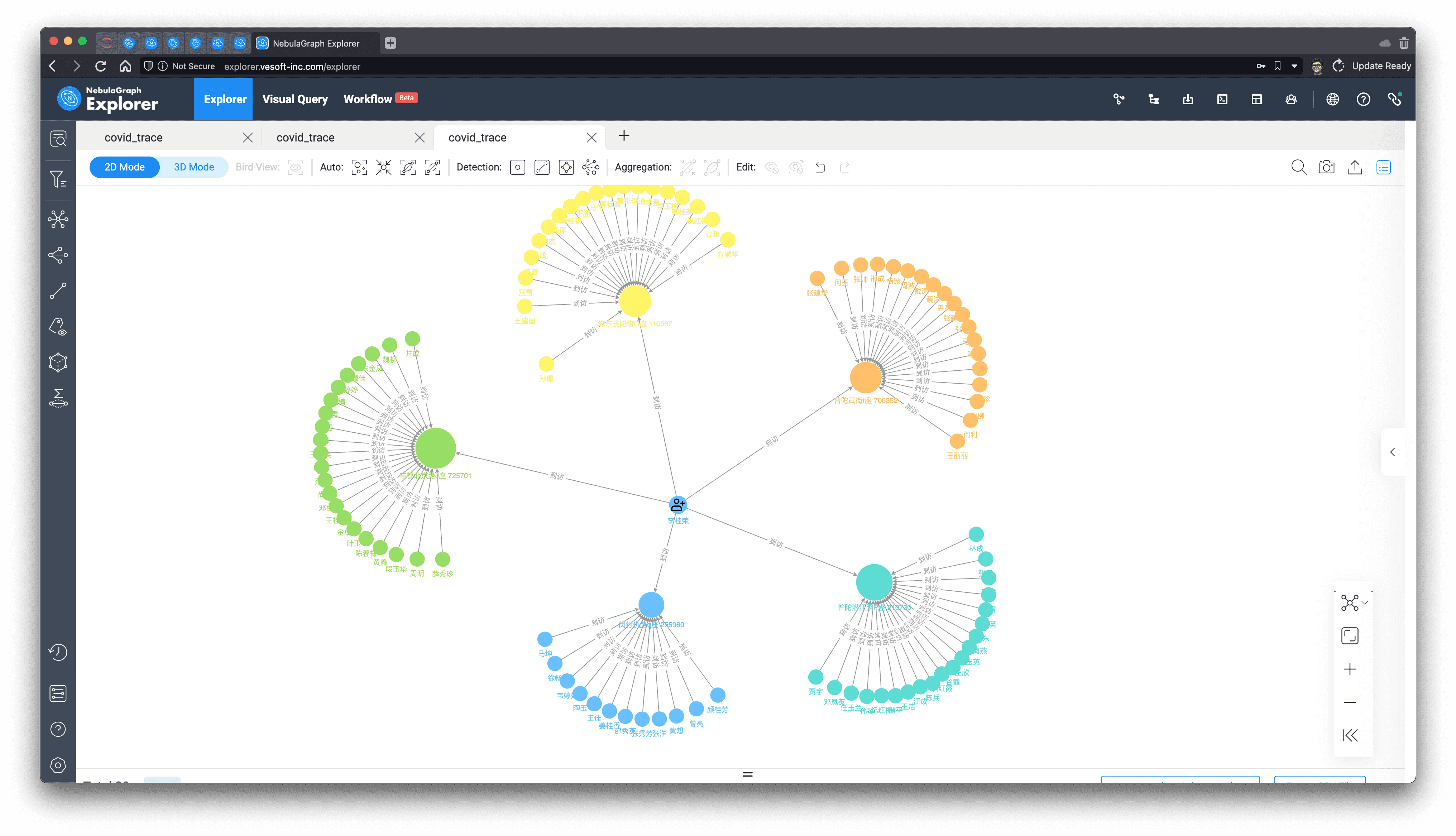
Now, let's visualize this result on a graph:

MATCH (p:person)-[`visit0`:visited]->(`addr`:address)<-[`visit1`:visited]-(p1:person)
    WHERE id(p) == "p_101" AND `visit0`.`start_time` < `visit1`.`end_time`
    RETURN paths;

In the result, we marked p_101 as a different icon, and identified the gathering community with the label propagation algorithm, isn't a graph worth a thousand words?

Most recently visited provinces

Finally, we then use a simple query pattern to express all the provinces a person has visited in a given time, say from a point in time:

MATCH (p:person)-[visit:visted]->(`addr`:address)-[:belong_to*5]-(prov:province)
    WHERE id(p) == "p_101" AND visit.start_time > 1625469000
    RETURN prov.province.name, collect(addr.address.name);

Result:

The usual rules, let's look at the results on the graph, this time, we choose Dagre-LR layout rendering, and the result looks like:

Recap

We have given quite a few examples of applications in social networks, including

• Finding key people
• Identifying clusters of people, communities
• Determining the closeness between two users
• Recommending new friends
• Pinpointing important content using common neighbors
• Push information flow based on friend relationship and geographic location
• Spatio-temporal relationship mapping

As a natural graph structure, social networks are well suited to use graph technology to store, query, compute, analyze and visualize to solve various problems on them. We hope you can have a preliminary understanding of the graph technology in SNS through this post.

How NebulaGraph Works

1. NebulaGraph Architecture — A Bird’s Eye View
2. Benchmark: NebulaGraph vs Dgraph vs JanusGraph
3. Comparison: Neo4j vs NebulaGraph vs JanusGraph
4. Deploy the Graph Database on Kubernetes